library(tidyverse)
library(tidymodels)Quantifying uncertainty
Application exercise
Answers
An article in the The Asheville Citizen-Times published in the summer of 2020 claims that the average price per guest (ppg) for properties in Asheville is $60 on Airbnb. To evaluate their claim we will use a dataset on 50 randomly selected Asheville Airbnb listings in June 2020. These data can be found in data/asheville.csv.
Let’s load the packages we’ll use first.
And then the data.
abb <- read_csv("data/asheville.csv")
glimpse(abb)
Rows: 50
Columns: 1
$ ppg <dbl> 48.00000, 40.00000, 99.00000, 13.00000, 55.00000, 75.00000, 74.000…Hypotheses
- Your turn: Write out the correct null and alternative hypothesis. Do this in both words and in proper notation.
Null hypothesis: The average price per guest (ppg) in Asheville is $60.
\[H_0: \mu = 60\]
Alternative hypothesis: The average price per guest (ppg) in Asheville is different than $60.
\[H_A: \mu \ne 60\]
Observed data
Our goal is to use calculate the probability of a sample statistic at least as extreme as the one observed in our data if in fact the null hypothesis is true.
- Demo: Calculate and report the sample statistic below using proper notation.
abb |>
  summarize(mean_ppg = mean(ppg))
# A tibble: 1 × 1
mean_ppg
<dbl>
1 76.6\[\bar{x} = 76.6\]
The null distribution
Let’s use simulation-based methods to conduct the hypothesis test specified above.
Generate
We’ll start by generating the null distribution.
- Demo: Generate the null distribution?
set.seed(4321)null_dist <- abb |>
specify(response = ppg) |>
hypothesize(null = "point", mu = 60) |>
generate(reps = 100, type = "bootstrap") |>
calculate(stat = "mean")- Your turn: Take a look at
null_dist. What does each element in this distribution represent?
null_distResponse: ppg (numeric)
Null Hypothesis: point
# A tibble: 100 × 2
replicate stat
<int> <dbl>
1 1 63.7
2 2 50.7
3 3 74.3
4 4 56.7
5 5 66.1
6 6 50.5
7 7 52.8
8 8 62.4
9 9 55.9
10 10 58.7
# … with 90 more rowsVisualize
- Question: Before you visualize the distribution of
null_dist– at what value would you expect this distribution to be centered? Why?
At 60, since we created this distribution assuming \(\mu = 60\).
- Demo: Create an appropriate visualization for your null distribution. Does the center of the distribution match what you guessed in the previous question?
ggplot(null_dist, aes(x = stat)) +
  geom_dotplot()
Bin width defaults to 1/30 of the range of the data. Pick better value with
`binwidth`.
- Demo: Now, add a vertical red line on your null distribution that represents your sample statistic.
ggplot(null_dist, aes(x = stat)) +
  geom_dotplot() +
  geom_vline(xintercept = 76.6, color = "red")
Bin width defaults to 1/30 of the range of the data. Pick better value with
`binwidth`.
- Question: Based on the position of this line, does your observed sample mean appear to be an unusual observation under the assumption of the null hypothesis?
Yes, it’s pretty far from the center.
p-value
Above, we eyeballed how likely/unlikely our observed mean is. Now, let’s actually quantify it using a p-value.
- Question: What is a p-value?
The probability of the observed sample statistic, or something more extreme in the direction of the alternative hypothesis, if in fact the null hypothesis is true.
- Demo: Visualize the p-value.
ggplot(null_dist, aes(x = stat)) +
  geom_dotplot() +
  geom_vline(xintercept = 76.6, color = "red") +
  geom_vline(xintercept = 43.4, color = "red", linetype = "dashed")
Bin width defaults to 1/30 of the range of the data. Pick better value with
`binwidth`.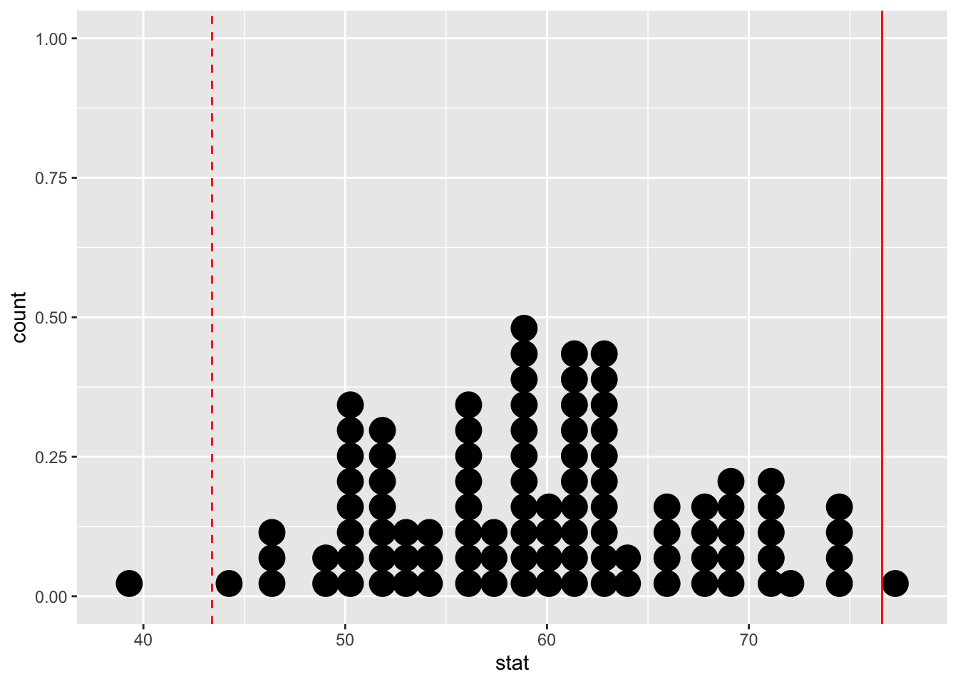
- Your turn: What is the p-value?
2/100 = 0.02.
Conclusion
- Your turn: What is the conclusion of the hypothesis test based on the p-value you calculated? Make sure to frame it in context of the data and the research question. Use a significance level of 5% to make your conclusion.
Since the p-value is smaller than the significance level, we reject the null hypothesis. The data provide convincing evidence that the average price per guest of properties on Airbnb in Asheville is different than $60.
- Demo: Interpret the p-value in context of the data and the research question.
If in fact the true average price per guest of properties on Airbnb in Ashevlle is $60, the probability of observing a random sample of 50 Asheville Airbnb listings where the average price per guest is $76.6 or higher or $43.4 or lower is 0.02.
Get real…
- Question: What we did above was a “toy example” to illustrate hypothesis test. What would you change to make this a real, more robust analysis?
Change the number of resamples to a higher number, somewhere ~10,000 replicates.
- Demo: Work through the analysis again with these changes.
null_dist <- abb |>
  specify(response = ppg) |>
  hypothesize(null = "point", mu = 60) |>
  generate(reps = 10000, type = "bootstrap") |>
  calculate(stat = "mean")

point_estimate <- abb |>
  specify(response = ppg) |>
  calculate(stat = "mean")

get_p_value(null_dist, point_estimate, direction = "two-sided")
# A tibble: 1 × 1
p_value
<dbl>
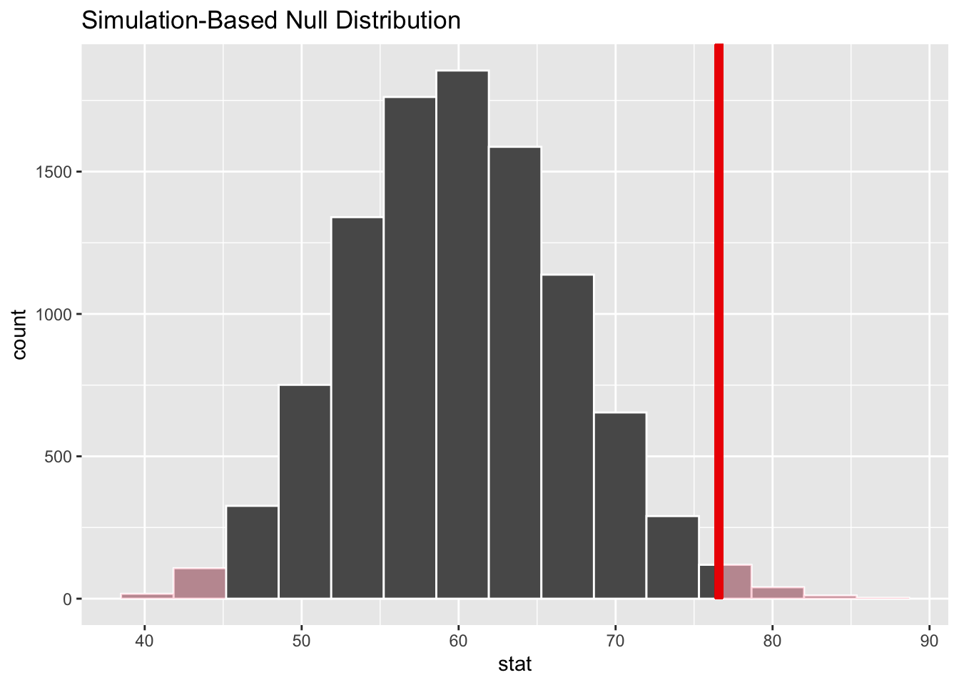
1 0.0246visualize(null_dist) +
shade_p_value(obs_stat = point_estimate, direction = "two-sided")