He replied / she cried: Text mining and gender roles

Application exercise

Answers

Important

These are suggested answers. This document should be used as reference only, it’s not designed to be an exhaustive key.

Introduction

Which verbs follow “she” and “he” pronouns in Jane Austen novels? Are they similar or different?

Goal: Use text mining methods to explore whether verbs that follow she and he pronouns are similar or different.

Inspirations:

Blog post by Julia Silge: https://juliasilge.com/blog/gender-pronouns
Jockers, Matthew, and Gabi Kirilloff. “Understanding gender and character agency in the 19th century novel.” Journal of Cultural Analytics 2.2 (2016): 11066.

Packages

library(tidyverse)

── Attaching packages ─────────────────────────────────────── tidyverse 1.3.2 ──
✔ ggplot2 3.4.0      ✔ purrr   0.3.5 
✔ tibble  3.1.8      ✔ dplyr   1.0.10
✔ tidyr   1.2.1      ✔ stringr 1.4.1 
✔ readr   2.1.3      ✔ forcats 0.5.2 
── Conflicts ────────────────────────────────────────── tidyverse_conflicts() ──
✖ dplyr::filter() masks stats::filter()
✖ dplyr::lag()    masks stats::lag()

library(tidytext)
library(knitr)
library(janeaustenr) # install.packages("janeaustenr)

Data

The janeaustenr package offers a function, austen_books(), that returns a tidy data frame of Jane Austen’s 6 completed, published novels.

austen_books <- austen_books() |>
  filter(text != "")

Demo: Which books are included in the dataset?

austen_books |>
  distinct(book)

# A tibble: 6 × 1
  book               
  <fct>              
1 Sense & Sensibility
2 Pride & Prejudice  
3 Mansfield Park     
4 Emma               
5 Northanger Abbey   
6 Persuasion

Word frequencies

Question: What would you expect to be the most common word in Jane Austen novels? Would you expect it to be the same across all books?

Answers may vary.

Demo: Split the text column into word tokens.

austen_words <- austen_books |>
  unnest_tokens(output = word, input = text) # token = "words" by default

Your turn: Discover the top 10 most commonly used words in each of Jane Austen’s books.

With stop words:

austen_words |>
  count(book, word, sort = TRUE) |>
  group_by(book) |>
  slice_head(n = 10) |>
  pivot_wider(
    names_from = book, 
    values_from = n,
    values_fn = as.character,
    values_fill = "Not in top 10"
    ) |>
  kable()

word	Sense & Sensibility	Pride & Prejudice	Mansfield Park	Emma	Northanger Abbey	Persuasion
to	4116	4162	5475	5239	2244	2808
the	4105	4331	6206	5201	3179	3329
of	3571	3610	4778	4291	2358	2570
and	3490	3585	5438	4896	2306	2800
her	2543	2203	3082	2462	1562	1203
a	2092	1954	3099	3129	1540	1594
i	1998	2065	2358	3177	1285	Not in top 10
in	1979	1880	2512	Not in top 10	1268	1389
was	1861	1843	2651	2398	1114	1337
it	1755	Not in top 10	2272	2528	1106	Not in top 10
she	Not in top 10	1695	Not in top 10	2340	Not in top 10	1146
had	Not in top 10	Not in top 10	Not in top 10	Not in top 10	Not in top 10	1187

Demo: Let’s do better, without the “stop words”.

stop_words

# A tibble: 1,149 × 2
   word        lexicon
   <chr>       <chr>  
 1 a           SMART  
 2 a's         SMART  
 3 able        SMART  
 4 about       SMART  
 5 above       SMART  
 6 according   SMART  
 7 accordingly SMART  
 8 across      SMART  
 9 actually    SMART  
10 after       SMART  
# … with 1,139 more rows

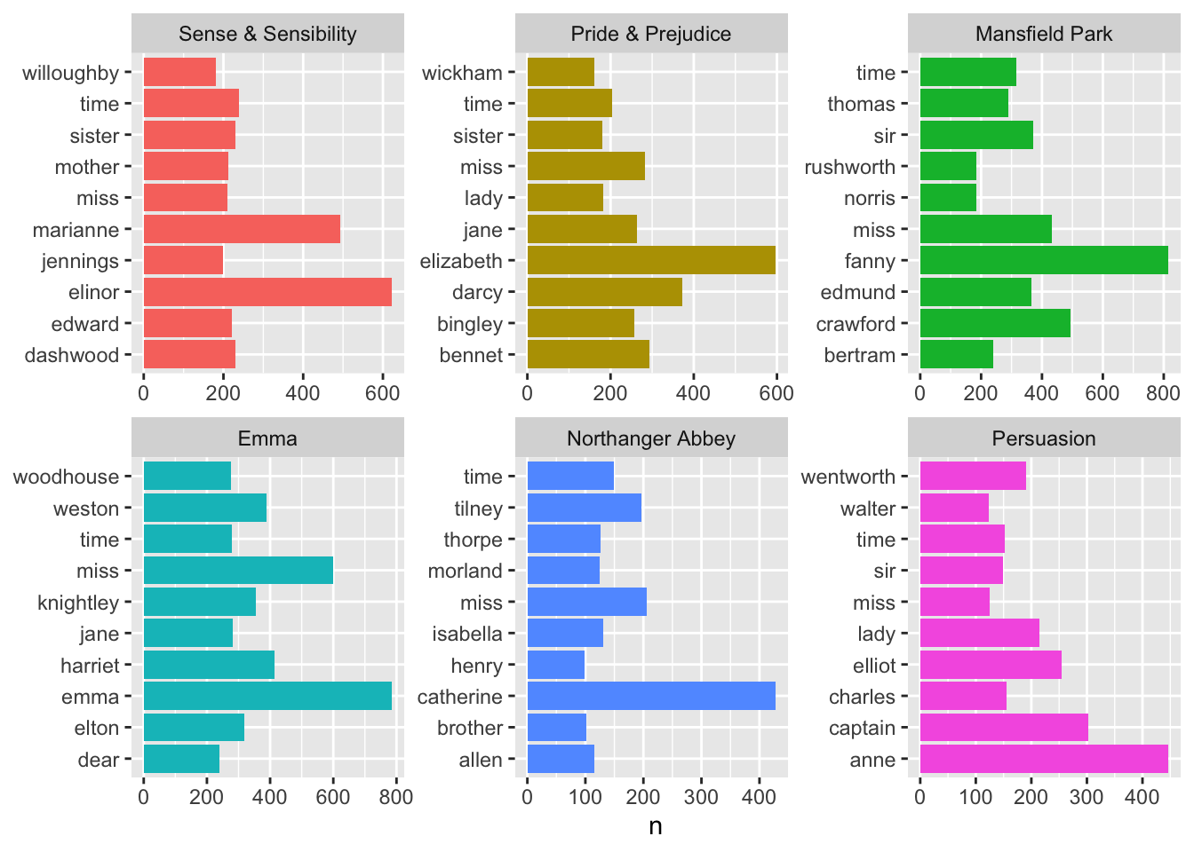
Without stop words:

austen_words |>
  anti_join(stop_words) |>
  count(book, word, sort = TRUE) |>
  group_by(book) |>
  slice_head(n = 10) |>
  ggplot(aes(y = word, x = n, fill = book)) +
  geom_col(show.legend = FALSE) +
  facet_wrap(~book, scales = "free") +
  labs(y = NULL)

Joining, by = "word"

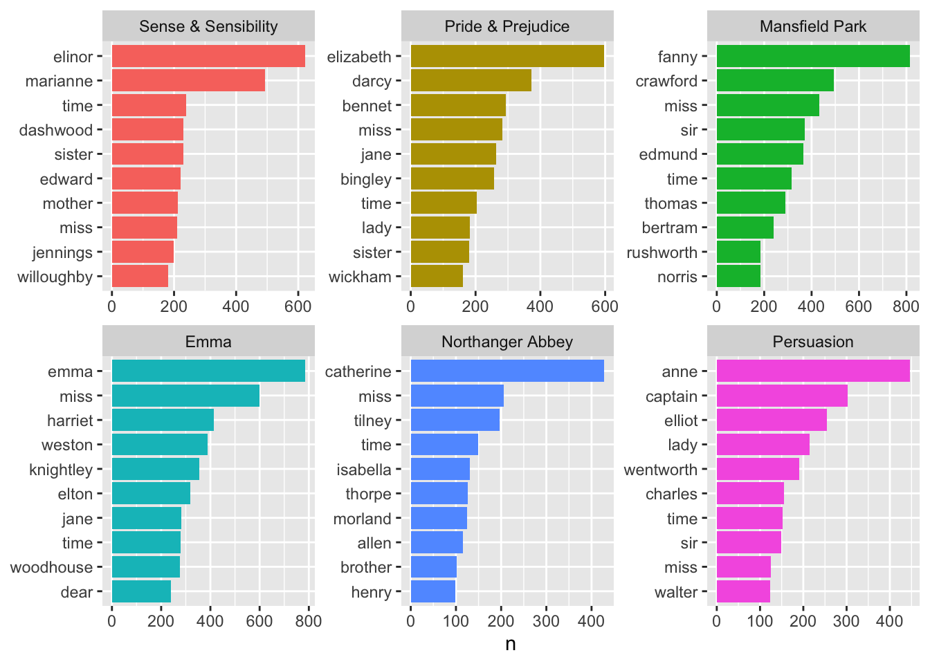
With better ordering:

austen_words |>
  anti_join(stop_words) |>
  count(book, word, sort = TRUE) |>
  group_by(book) |>
  slice_head(n = 10) |>
  ggplot(aes(y = reorder_within(word, n, book), x = n, fill = book)) +
  geom_col(show.legend = FALSE) +
  facet_wrap(~book, scales = "free") +
  scale_y_reordered() +
  labs(y = NULL)

Joining, by = "word"

Bigram frequencies

An n-gram is a contiguous series of \(n\) words from a text; e.g., a bigram is a pair of words, with \(n = 2\).

Demo: Split the text column into bigram tokens.

austen_bigrams <- austen_books |>
  unnest_tokens(bigram, text, token = "ngrams", n = 2) |>
  filter(!is.na(bigram))

austen_bigrams

# A tibble: 662,783 × 2
   book                bigram         
   <fct>               <chr>          
 1 Sense & Sensibility sense and      
 2 Sense & Sensibility and sensibility
 3 Sense & Sensibility by jane        
 4 Sense & Sensibility jane austen    
 5 Sense & Sensibility chapter 1      
 6 Sense & Sensibility the family     
 7 Sense & Sensibility family of      
 8 Sense & Sensibility of dashwood    
 9 Sense & Sensibility dashwood had   
10 Sense & Sensibility had long       
# … with 662,773 more rows

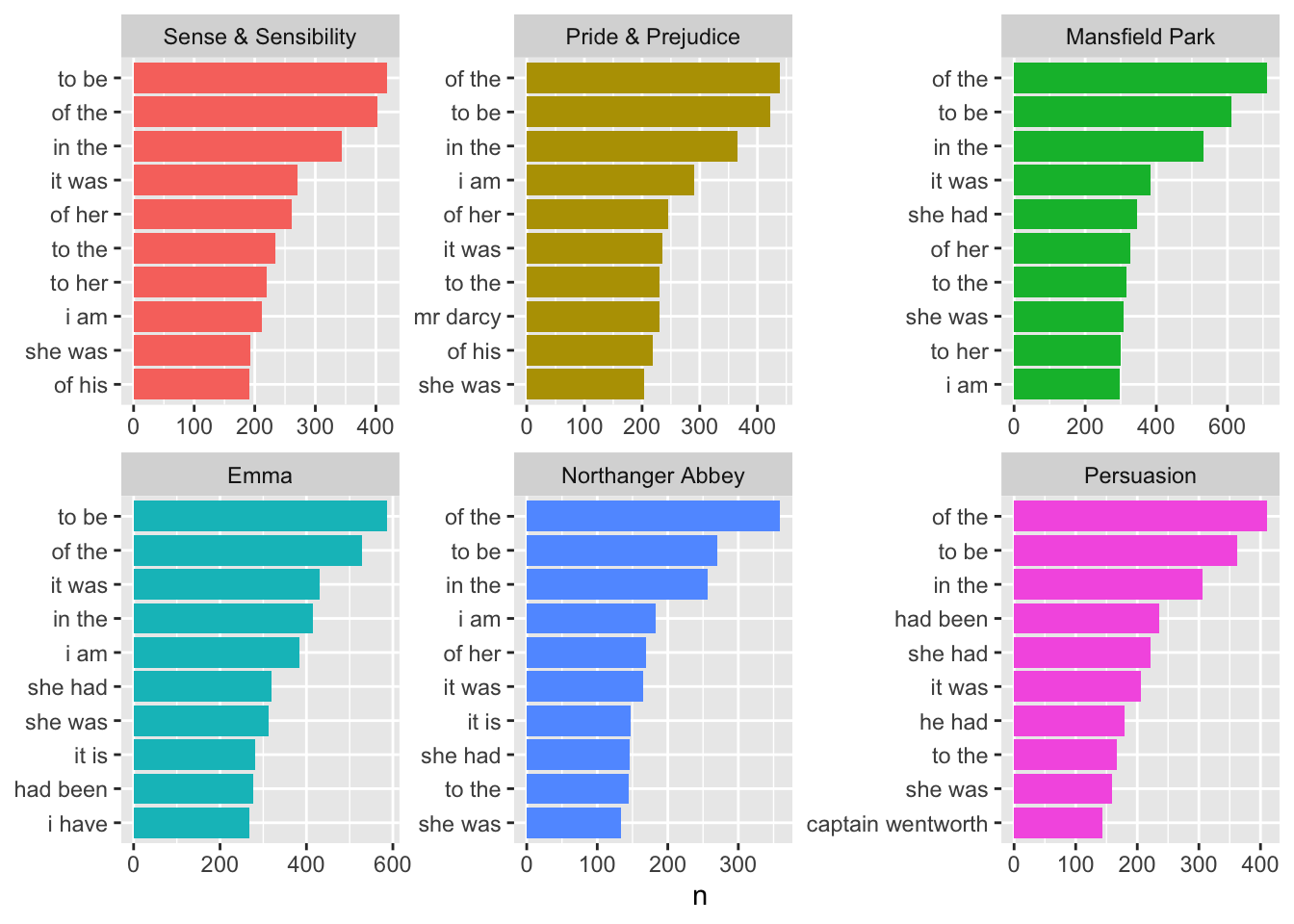
Your turn: Visualize the frequencies of top 10 bigrams in each of Jane Austen’s books.

austen_bigrams |>
  count(book, bigram, sort = TRUE) |>
  group_by(book) |>
  slice_head(n = 10) |>
  ggplot(aes(y = reorder_within(bigram, n, book), x = n, fill = book)) +
  geom_col(show.legend = FALSE) +
  facet_wrap(~book, scales = "free") +
  scale_y_reordered() +
  labs(y = NULL)

Verbs that follow she or he

First, let’s define the pronouns of interest:

pronouns <- c("he", "she")

Demo: Filter the dataset for bigrams that start with either “she” or “he” and calculate the number of times these bigrams appeared.

bigram_counts <- austen_bigrams |>
  count(bigram, sort = TRUE) |>
  separate(bigram, into = c("word1", "word2"), sep = " ") |>
  filter(word1 %in% pronouns) |>
  count(word1, word2, wt = n, sort = TRUE) |>
  rename(total = n)

bigram_counts

# A tibble: 1,490 × 3
   word1 word2 total
   <chr> <chr> <int>
 1 she   had    1405
 2 she   was    1309
 3 he    had     965
 4 he    was     844
 5 she   could   767
 6 he    is      385
 7 she   would   348
 8 she   is      311
 9 he    could   281
10 he    would   244
# … with 1,480 more rows

Discussion: What can we do next to see if there is a difference in the types of verbs that follow “he” vs. “she”?

Answers may vary.

Demo: Which words have about the same likelihood of following “he” or “she” in Jane Austen’s novels?

word_ratios <- bigram_counts |>
  group_by(word2) |>
  filter(sum(total) > 10) |>
  ungroup() |>
  pivot_wider(names_from = word1, values_from = total, values_fill = 0) |>
  arrange(word2) |>
  mutate(
    she = (she+1)/sum(she+1),
    he = (he+1)/sum(he+1),
    logratio = log(she / he, base = 2)
  ) |>
  arrange(desc(logratio))

word_ratios

# A tibble: 158 × 4
   word2          she       he logratio
   <chr>        <dbl>    <dbl>    <dbl>
 1 remembered 0.00167 0.000165     3.34
 2 read       0.00274 0.000495     2.47
 3 resolved   0.00131 0.000330     1.99
 4 felt       0.0216  0.00577      1.90
 5 longed     0.00167 0.000495     1.75
 6 received   0.00214 0.000659     1.70
 7 feared     0.00238 0.000824     1.53
 8 dared      0.00274 0.000989     1.47
 9 heard      0.00500 0.00181      1.46
10 tried      0.00226 0.000824     1.46
# … with 148 more rows

word_ratios |> 
  arrange(abs(logratio))

# A tibble: 158 × 4
   word2         she       he logratio
   <chr>       <dbl>    <dbl>    <dbl>
 1 ought    0.00548  0.00561   -0.0330
 2 walked   0.00369  0.00379   -0.0385
 3 would    0.0416   0.0404     0.0413
 4 loves    0.000953 0.000989  -0.0541
 5 too      0.000953 0.000989  -0.0541
 6 paused   0.00155  0.00148    0.0614
 7 turned   0.00310  0.00297    0.0614
 8 very     0.00155  0.00148    0.0614
 9 had      0.167    0.159      0.0724
10 listened 0.00226  0.00214    0.0784
# … with 148 more rows

Demo: Which words have different likelihoods of following “he” or “she” in Jane Austen’s novels?

word_ratios |>
  mutate(abslogratio = abs(logratio)) |>
  group_by(logratio < 0) |>
  top_n(15, abslogratio) |>
  ungroup() |>
  mutate(word = reorder(word2, logratio)) |>
  ggplot(aes(word, logratio, color = logratio < 0)) +
  geom_segment(
    aes(
      x = word, xend = word,
      y = 0, yend = logratio
    ),
    linewidth = 1.1, alpha = 0.6
  ) +
  geom_point(size = 3.5) +
  coord_flip() +
  labs(
    x = NULL,
    y = "Relative appearance after 'she' compared to 'he'",
    title = "Words paired with 'he' and 'she' in Jane Austen's novels",
    subtitle = "Women remember, read, and feel while men stop, take, and reply"
  ) +
  scale_color_discrete(name = "", labels = c("More 'she'", "More 'he'")) +
  scale_y_continuous(
    breaks = seq(-3, 3),
    labels = c(
      "0.125x", "0.25x", "0.5x",
      "Same", "2x", "4x", "8x"
    )
  )

Sentiment analysis

One way to analyze the sentiment of a text is to consider the text as a combination of its individual words and the sentiment content of the whole text as the sum of the sentiment content of the individual words. This isn’t the only way to approach sentiment analysis, but it is an often-used approach, and an approach that naturally takes advantage of the tidy tool ecosystem.¹

sentiments <- get_sentiments("afinn")
sentiments

# A tibble: 2,477 × 2
   word       value
   <chr>      <dbl>
 1 abandon       -2
 2 abandoned     -2
 3 abandons      -2
 4 abducted      -2
 5 abduction     -2
 6 abductions    -2
 7 abhor         -3
 8 abhorred      -3
 9 abhorrent     -3
10 abhors        -3
# … with 2,467 more rows

bigram_counts |>
  left_join(sentiments, by = c("word2" = "word")) |>
  filter(!is.na(value)) |>
  mutate(sentiment = total * value) |>
  group_by(word1) |>
  arrange(desc(abs(sentiment))) |>
  slice_head(n = 10)

# A tibble: 20 × 5
# Groups:   word1 [2]
   word1 word2      total value sentiment
   <chr> <chr>      <int> <dbl>     <dbl>
 1 he    loved         16     3        48
 2 he    cried         11    -2       -22
 3 he    liked         10     2        20
 4 he    trusted        8     2        16
 5 he    bore           7    -2       -14
 6 he    smiling        7     2        14
 7 he    stopped       13    -1       -13
 8 he    delighted      4     3        12
 9 he    likes          5     2        10
10 he    smiled         5     2        10
11 she   cried         44    -2       -88
12 she   loved         17     3        51
13 she   liked         17     2        34
14 she   trusted       13     2        26
15 she   resolved      10     2        20
16 she   rejoiced       5     4        20
17 she   likes          8     2        16
18 she   lost           5    -3       -15
19 she   determined     6     2        12
20 she   dreaded        6    -2       -12

Footnotes

Tidy Text Mining: https://www.tidytextmining.com/sentiment.html.↩︎